1. What is Dijkstra's Algorithm?

Dijkstra's Shortest Path Algorithm, or just known as djikstra, is an algorithm that is able to find the shortest path on a weighted graph. This is different from BFS where the graph must be unweighted. Dijkstra is able to work on graphs with non-uniform weights, and thus is much more useful in the real world. However, this comes at a cost of the performance of the algorithm. Previously, BFS has a time complexity of O(E + N), which means the time the algorithm takes scales linearly with input. Dijkstra, however, has a time complexity of O(E*log(N)), meaning that it still scales linearly, but now has a logarithmic factor. Note: In time complexity analysis, the base of the log does not matter.

2. Applications of Dijkstra's Algorithm

As we have previously discussed for BFS, graph search algorithms are able to traverse through graphs. With dijkstra, we are now able to find the paths on weighted nodes. With this newfound power, we are now able to enter the real world. With weighted edges, it is now possible to map real-world points into nodes, and find the distances between them. Think about the path finding algorithm used in car navigation. It needs to be able to determine a route in non-trival scenarios. For example, the distance between two intersections could be a different, meaning that taking one edge could result in a shorter distance than another. With dijkstra, it is possible to simply express the distance travelled between intersections as different weights on two edges.

3. How does Dijkstra's Algorithm work?

Dijkstra works in a similar way to BFS. Dijkstra searches adjacent nodes, and visits them. But compared to BFS, dijkstra visits the nodes in a different order. It searches through the graph greedily by visiting the node with the shortest distance first. Additionally, dijkstra introduces a new concept called edge relaxation. Edge relaxation repeatedly minimizes the path to a certain node until it is optimal. When a node is considered as visited, the node propagates its own weights to the surrounding nodes. If the weight from the starting node S to the current node C + the weight of the edge from C to the adjacent node A is more optimal than the path from S to A, then node A's path can be rerouted through C to attain a better answer. This process of relaxing the edges and visiting shortest nodes is repeated until all nodes and paths are exhausted. At the end, the minimal path is achieved.

4. A visual demonstration

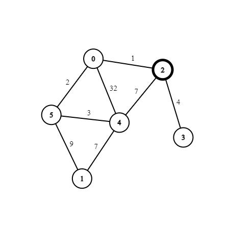
Here is the graph that is shown on the homepage. We will run Dijkstra's algorithm to find the shortest path between nodes 1 and 3

Initial State

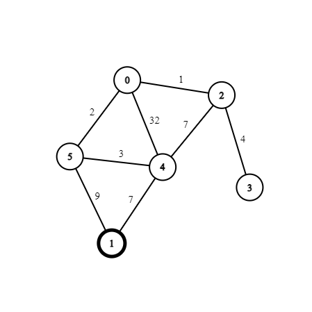
We will start off at node 1, and explore our neighbours. Here is our current state:

Node	0	1	2	3	4	5
Distance	∞	0	∞	∞	∞	∞

Explore Node 1's Neighbours

Node	0	1	2	3	4	5
Distance	∞	0	∞	∞	7	9

Queue	{Node=4, Dist=7}	{Node=5, Dist=9}

Visit Node 4 & Explore Neighbours

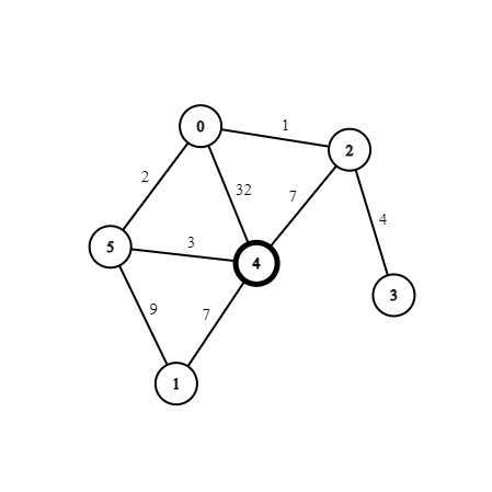
Notice, node 5 is not visited from node 4 because 7 + 3 > 9

Node	0	1	2	3	4	5
Distance	39	0	14	∞	7	9

Queue	{Node=5, Dist=9}	{Node=2, Dist=14}	{Node=0, Dist=39}

Visit Node 5 & Explore Neighbours

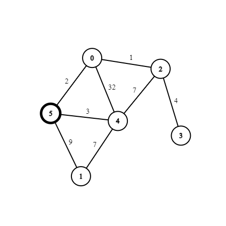
Notice, node 4 is not visited because 9 + 3 > 7. Additionally, we have found a shorter path to node 0 through edge relaxation. 9 + 2 < 7 + 32.

Node	0	1	2	3	4	5
Distance	11	0	14	∞	7	9

Queue	{Node=0, Dist=11}	{Node=2, Dist=14}	{Node=0, Dist=39}

Visit Node 0 & Explore Neighbours

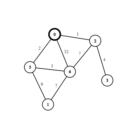
In this iteration, we have found a shorter path to node 2 through node 0. We do not visit node 4 because 11 + 32 > 7.

Node	0	1	2	3	4	5
Distance	11	0	12	∞	7	9

Queue	{Node=2, Dist=12}	{Node=2, Dist=14}

Visit Node 2 & Explore Neighbours

We have found our ending node, but we should still iterate until our queue is empty. This ensures that we truly have the shortest path.

Node	0	1	2	3	4	5
Distance	11	0	12	16	7	9

Queue	{Node=3, Dist=16}

Visit Node 3 & Explore Neighbours

At node 3, we can no longer discover any further paths, and the algorithm terminates.

Node	0	1	2	3	4	5
Distance	11	0	12	16	7	9

Queue	Empty

5. An interesting observation

Phew, that was a lot of typing. Hopefully you followed along. But there are some interesting observations... Can you spot them? —Well, I will show them to you anyways.

1. The nodes are never visited again once they are taken from the queue, meaning that once a node is at the front of the queue, the distance is already determined.

2. Notice the distance array. It turns out that Dijkstra's algorithm actually finds the minimal distance to ALL nodes. This can be helpful in reducing re-calculations when calculating the distance from a fixed source.

6. Next steps?

In order to use a path-finding algorithm in the real world, it needs to be able to handle the massive amount of data that the world stores. Think about how many intersections there are in a city. Dijkstra simply is not fast enough to power the navigation tools that we rely on. This is where heuristic algorithms come in to save the day.

Footnote

Thanks Mr. Benum for correcting an error on this page!